Data Transformation (Statistics)

The scattering diagram in which the areas of sovereign states and dependent territories in the world are plotted along the vertical axis relative to the population of these countries, plotted along the horizontal axis. The top chart uses raw data. In the lower graph, the areas and populations are transformed using a logarithmic function.

Data transformation is the application of a deterministic mathematical function to each point of a data set, that is, each data point z _i is replaced by a converted value $y_{i}=f(z_{i})$ ${\ displaystyle y_ {i} = f (z_ {i})}$ ${\ displaystyle y_ {i} = f (z_ {i})}$ where f is a function. Transformations are usually applied so that the data is more suitable for the statistical inference procedure that you want to apply, to improve interpretability, or for representation.

Almost always, the function that is used to transform the data is reversible , and usually continuous . Conversion is usually applied to a collection of comparable metrics. For example, if we work with data on people's incomes in a certain currency , the income of each person is usually converted using a logarithmic function.

Content

Motivation

Guidance on how data should be transformed or whether it should be transformed at all should come from a specific statistical analysis. For example, a simple way to construct an approximately 95% confidence interval for the mathematical expectation of a population is to take the arithmetic mean plus or minus two standard errors . However, the constant factor 2 used here refers to the normal distribution and is applicable only if the arithmetic mean varies approximately according to the normal law. The central limit theorem states that in many situations the arithmetic mean does not vary according to the normal law if the sample size is large enough. However, if the population is substantially asymmetric and the sample size is moderate, the approximation given by the central limit theorem may be poor, and the resulting confidence interval will most likely have the wrong . Then, in the case when there is evidence of a significant asymmetry of the data, usually the data is converted to a symmetric distribution before constructing a confidence interval. If necessary, the confidence interval can be converted back to the original scale, using the inverse to that used for data conversion.

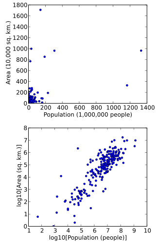
Data can also be converted to facilitate visualization. For example, suppose we have a scatter chart in which the points are the countries of the world, and the data values shown on the graph reflect the area and population of each country. If the graph is made from non-transformed data (for example, square kilometers for the area and the number of people in the population), most countries will end up in a dense cluster in the lower left corner of the graph. Some countries with a very large area and / or population will be distributed liquidly over the main area of the schedule. Simple scaling of units (for example, to thousands of square kilometers or to millions of people) does not change the situation. However, during the logarithmic transformation of both area and population, points will be distributed more evenly on the graph.

The final reason for data conversion may be improved interpretability, even if no formal statistical analysis or visualization is intended. For example, suppose we compare cars in terms of their fuel economy. These data are usually presented as “kilometers per liter” or “miles per gallon”. However, if the goal is to determine how much extra fuel per person you need to use per year, if you use one car compared to another, it is more natural to work with data converted using the 1 / x function, which gives liters per kilometer or gallons per mile.

In Regression

Linear regression is a statistical technique for linking the dependent variable Y with the more or less independent variables X. The simplest regression models reveal a linear relationship between the mathematical expectation of Y and each independent variable (if other independent variables are fixed). If linearity is not fulfilled, even approximately, sometimes it is possible to transform either independent variables or dependent variables in a regression model to improve linearity.

Another assumption of linear regression is that the variance is the same for any possible mathematical expectation (which is known as homoskedasticity ). One-dimensional normality is not necessary for the least squares estimation of the regression parameters to make sense (see the article “ Gauss – Markov Theorem ”). However, confidence intervals and hypothesis testing will have better statistical properties if the variables have multidimensional nominality. This can be obtained empirically by graphically representing the values with respect to the and examining the residuals. Note, it doesn’t matter if the dependent variable Y is normally distributed or not.

Alternative

OL] provides a flexible generalization of conventional linear regression, which makes it possible to output variables that have error distribution models other than the normal distribution. OLM allows the linear model to be associated with output variables using the communication function and allows the variance of each measurement to be a function of the calculated value.

Examples

The equation: $Y=a+bX$ ${\ displaystyle Y = a + bX}$

Value: A single increase in X is associated on average with an increase in b times the value of Y.

Equality: $\log(Y)=a+bX$ ${\ displaystyle \ log (Y) = a + bX}$ (Obtained by taking the logarithm from both sides of the equality $Y=e^{a}e^{bX}$ ${\ displaystyle Y = e ^ {a} e ^ {bX}}$ )

Value: A single increase in X is associated, on average, with a b% increase in Y.

Equality: $Y=a+b\log(X)$ ${\ displaystyle Y = a + b \ log (X)}$

Value: An increase of 1% X is associated with an average increase in b / 100 times the value of Y.

Equality: $\log(Y)=a+b\log(X)$ ${\ displaystyle \ log (Y) = a + b \ log (X)}$ (Obtained by taking the logarithm from both sides of the equality $Y=e^{a}X^{b}$ ${\ displaystyle Y = e ^ {a} X ^ {b}}$ )

Value: An increase of 1% X is associated with an average increase in b% of Y.

General cases

Logarithmic transforms and square root transformations are usually used for positive data, and conversion to the opposite in multiplication (1 / x) can be used for non-zero data. is a family of transformations parameterized by a non-negative value of λ, this family includes the logarithmic transformation, the square root transformation, and the inverse value transformation (1 / x) as special cases. To get the data transformation purposefully, you can use the statistical estimation technique to estimate the parameter λ in a power-law transformation, thereby determining the transformation that is most suitable under given conditions. Since the power transformation family also includes the identity transformation, this approach can also show whether it is better to analyze data without conversion. In a regression analysis, this technique is known as the Box-Cox technique.

Converting to the opposite value (1 / x) and some power transforms can be successfully applied to data that contains both positive and negative values (the power transform is invertible for all real numbers if λ is an odd integer). However, if both positive and negative values are observed, they usually start by adding a constant to all the values to obtain a set of non-negative numbers, to which any power transformation can then be applied. The usual situation when data transformation is applied is when the spread of the considered values is several orders of magnitude . Many physical and social phenomena exhibit this behavior — income, population size, galaxy size, and rainfall as examples. A power transformation, and in particular a logarithm, can often be used to achieve symmetry in such data. The logarithm is often preferable because it is easier to interpret its results in terms of the “multiplicity of changes”.

The logarithm also has a useful property on fractions. If we compare the positive values of X and Y using the X / Y ratios, then in the case X < Y, the ratio falls on the unit interval (0,1), and when X > Y , the ratio falls on the semi-axis (1, ∞), and the equality of the ratio 1 corresponds to the equality of values. In the analysis, when X and Y are treated symmetrically, the logarithm of the relation log ( X / Y ) is equal to zero in the case of equality and there is a property that in the case when X is K times greater than Y , the logarithm of the ratio is equally non-zero from the case when Y is K times greater than X (the logarithm of the ratio in these situations is log ( K ) and −log ( K )).

If the values initially lie between 0 and 1, not including the boundary values, then the logit transformation may be suitable - it gives values in the range (−∞, ∞).

Converting to Normal Distribution

It is not always necessary or desirable to convert the data set to a normal distribution. However, if symmetry or normality is desired, often this can be done using one of the power transformations.

To assess whether we have achieved normality, the graphical approach is often more informative than the formal statistical test. Commonly used to evaluate whether we have a normally distributed population, . Alternatively, universal rules are used, based on the example of asymmetry and kurtosis , when the asymmetry reaches a value from −0.8 to 0.8, and the kurtosis lies in the range from −3.0 to 3.0.

Convert to a uniform or arbitrary distribution

If we observe a set of n values $X_{1},\dots ,X_{n}$ ${\ displaystyle X_ {1}, \ dots, X_ {n}}$ without coincidence (i.e., all n values are different), we can replace X _i with the converted value $Y_{i}=k$ ${\ displaystyle Y_ {i} = k}$ , where k is determined so that X _i is the k- th largest value among all X values. This is called a ranking transformation and it creates data that is ideally compatible with uniform distribution .

When using the , if X is any random variable , and F is a cumulative distribution function of X , then, in the case of F reversibility, the random variable U = F ( X ) will satisfy the uniform distribution on the unit interval [0, one].

We can transform a homogeneous distribution to any distribution using the reversible cumulative distribution function. If G is a reversible cumulative distribution function, and U is a uniformly distributed random variable, then the random variable $G^{-1}(U)$ ${\ displaystyle G ^ {- 1} (U)}$ has G as a cumulative distribution function.

That is, if X is any random variable, F is a reversible cumulative distribution function of X , and G is a reversible cumulative distribution function, then the random variable $G^{-1}(F(X))$ ${\ displaystyle G ^ {- 1} (F (X))}$ has G as a cumulative distribution function.

Dispersion Stabilizing Transformations

Many types of statistical data exhibit a relationship of “ variance and average”, which means that variability is different for data values with different mathematical expectations . As an example, when comparing different populations in the world, an increase in the dispersion of income leads to an increase in the mathematical expectation of income. If we look at the number of small units of area (for example, administrative districts in the United States of America) and get the average and variance of incomes for each district, we usually get that districts with large average incomes have a big variance.

is aimed at removing the relationship between dispersion and mathematical expectation, so that the variance becomes constant relative to the average. Examples of variance stabilizing are for a sample correlation coefficient, the square root or for data obeying the Poisson distribution (discrete data), for regression analysis, and conversion to arcsine from the square root or trigonometric transformation for proportions ( binomial data). The transformation to the square root arcsine usually used for statistical analysis of proportional data is not recommended, since logistic regression or logit transformation are more suitable for binomial or non-binomial proportions, respectively, especially in view of the reduction of type II errors ^[1] .

Transformations for Multidimensional Statistics

One-dimensional functions can be applied pointwise to multidimensional data to change their private distributions. It is also possible to change some properties of multidimensional distributions using suitably constructed transformations. For example, when working with time series and other types of serial data, they usually move to finite data differences to improve stationarity . If the data formed by the random vector X are observed as observation vectors X _i with the covariance matrix Σ, a linear mapping can be used to eliminate the correlation of the data. To do this, use the Cholesky decomposition to obtain Σ = A A ' . Then the transformed vector $Y_{i}=A^{-1}X_{i}$ ${\ displaystyle Y_ {i} = A ^ {- 1} X_ {i}}$ has an identity matrix as a covariance matrix.

Notes

↑ Warton, Hui, 2011 , p. 3-10.

Literature

Warton D., Hui F. The arcsine is asinine: the analysis of proportions in ecology // Ecology. - 2011 .-- T. 92 . - DOI : 10.1890 / 10-0340.1 .

Links

Log transformation
Transformations, means, and confidence intervals
Log Transformations for Skewed and Wide Distributions - discusses the logarithmic and “signed logarithmic” transformations (Chapter from “Practical Data Science with R”).

[_149215905fcd51c7-1] Warton, Hui, 2011 , p. 3-10.