Plane wave

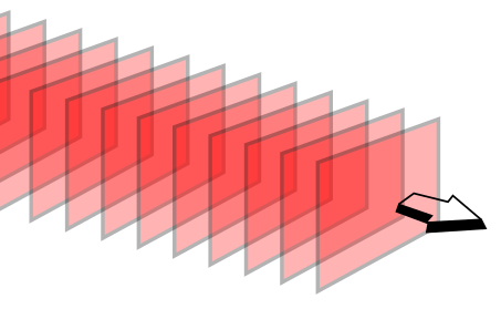
Fronts of a plane wave in three-dimensional space and the phase velocity vector

A plane wave is a wave whose front is flat.

The front of a plane wave is unlimited in size, the phase velocity vector is perpendicular to the front.

A plane wave is a particular solution of the wave equation and a convenient theoretical model : such a wave does not exist in nature, since the plane wave front begins at $-{\mathcal {\infty }}$ ${\ displaystyle - {\ mathcal {\ infty}}}$ ${\ displaystyle - {\ mathcal {\ infty}}}$ and ends in $+{\mathcal {\infty }}$ ${\ displaystyle + {\ mathcal {\ infty}}}$ ${\ displaystyle + {\ mathcal {\ infty}}}$ which obviously cannot be. Such a wave would carry infinite power , and infinite energy would be required to create a wave. The convenience of a plane wave model is due to the fact that a wave with a complex (real) front can be represented as a superposition ( spectrum ) of plane waves using the Fourier transform with respect to spatial variables.

A quasiplane wave is a wave whose front is close to plane in a certain limited region. If the size of the region is large enough for the characteristic size of the phenomenon, then the quasi-plane wave can be approximately considered flat. A wave with a complex front can be approximated by the sum of local quasi-plane waves whose phase velocity vectors are normal to the real front at each of its points. Examples of sources of quasi-plane electromagnetic waves are a laser , a mirror and a lens antenna : the distribution of the phase of the electromagnetic field in a plane parallel to the aperture (radiating hole) is close to uniform. As you move away from the aperture, the wave front takes on a complex shape.

Content

Definition

The equation of any wave is a solution to a differential equation called the wave equation . Wave equation for function $A$ ${\ displaystyle A}$ $A$ written as

\Delta A({\vec {r}},t)={\frac {1}{v^{2}}}\,{\frac {\partial ^{2}A({\vec {r}},t)}{\partial t^{2}}},

{\ displaystyle \ Delta A ({\ vec {r}}, t) = {\ frac {1} {v ^ {2}}} \, {\ frac {\ partial ^ {2} A ({\ vec { r}}, t)} {\ partial t ^ {2}}},}

\Delta A({\vec {r}},t)={\frac {1}{v^{2}}}\,{\frac {\partial ^{2}A({\vec {r}},t)}{\partial t^{2}}},

Where

\Delta

{\ displaystyle \ Delta}

\Delta

- Laplace operator ;

A({\vec {r}},t)

{\ displaystyle A ({\ vec {r}}, t)}

A(\vec{r},t)

- desired function;

r

{\ displaystyle r}

r

Is the radius vector of the desired point;

v

{\ displaystyle v}

v

- wave speed;

t

{\ displaystyle t}

t

- time.

One-dimensional case

In this animated image, the coordinate is plotted along the horizontal axis

x

{\ displaystyle x}

in space, vertically - the value of an oscillating physical quantity

A

{\ displaystyle A}

, forming a wave with a harmonic dependence on time, at each point in space at the current moment in time. Blue line - spatial dependence graph

A(x)

{\ displaystyle A (x)}

physical quantity at the current time

t=t_{1},t_{2},...

{\ displaystyle t = t_ {1}, t_ {2}, ...}

The dependence on the coordinate is also harmonic. Shifting to the right over time, the graph

A(x)

{\ displaystyle A (x)}

coincides with itself at the previous moment in time - a wave process. The blue circle represents the wobble.

A(t)

{\ displaystyle A (t)}

physical quantity

A

{\ displaystyle A}

at one of the points along the coordinate

x=x_{0}.

{\ displaystyle x = x_ {0}.}

Plane Wave Motion Animation

In the one-dimensional case, the wave equation takes the form:

{\frac {\partial ^{2}A({\vec {r}},t)}{\partial x^{2}}}={\frac {1}{v^{2}}}\,{\frac {\partial ^{2}A({\vec {r}},t)}{\partial t^{2}}},

{\ displaystyle {\ frac {\ partial ^ {2} A ({\ vec {r}}, t)} {\ partial x ^ {2}}} = {\ frac {1} {v ^ {2}} } \, {\ frac {\ partial ^ {2} A ({\ vec {r}}, t)} {\ partial t ^ {2}}},}

Where

x

{\ displaystyle x}

- coordinate.

A particular solution to this equation for a plane harmonic wave :

A(x,t)=A_{o}\cos \left(kx-\omega t+\varphi _{0}\right),

{\ displaystyle A (x, t) = A_ {o} \ cos \ left (kx- \ omega t + \ varphi _ {0} \ right),}

Where

A(x,t)

{\ displaystyle A (x, t)}

- the magnitude of the perturbation at a given point in space

x

{\ displaystyle x}

and at time

t

{\ displaystyle t}

;

A_{o}

{\ displaystyle A_ {o}}

- wave amplitude ;

k

{\ displaystyle k}

- wave number ;

\omega

{\ displaystyle \ omega}

- circular frequency ;

\varphi _{0}

{\ displaystyle \ varphi _ {0}}

- the initial phase of the oscillations .

The wave number is expressed:

k={\frac {2\pi }{\lambda }},

{\ displaystyle k = {\ frac {2 \ pi} {\ lambda}},}

Where

\lambda

{\ displaystyle \ lambda}

- the spatial period of the change in the function of the wavelength .

The circular frequency of oscillation is expressed:

\omega ={\frac {2\pi }{T}}=2\pi f,

{\ displaystyle \ omega = {\ frac {2 \ pi} {T}} = 2 \ pi f,}

Where

T

{\ displaystyle T}

- period of fluctuations ;

f

{\ displaystyle f}

- frequency of oscillation.

When substituting in the expression for the wave of these expressions, the wave can also be described by the expressions:

A=A_{o}\cos \left[2\pi \left({\cfrac {x}{\lambda }}-{\cfrac {t}{T}}\right)+\varphi _{0}\right],

{\ displaystyle A = A_ {o} \ cos \ left [2 \ pi \ left ({\ cfrac {x} {\ lambda}} - {\ cfrac {t} {T}} \ right) + \ varphi _ { 0} \ right],}

or:

A=A_{o}\cos \left[2\pi \left({\cfrac {x}{\lambda }}-ft\right)+\varphi _{0}\right],

{\ displaystyle A = A_ {o} \ cos \ left [2 \ pi \ left ({\ cfrac {x} {\ lambda}} - ft \ right) + \ varphi _ {0} \ right],}

or:

A=A_{o}\cos \left[{\cfrac {2\pi }{\lambda }}(x-vt)+\varphi _{0}\right],

{\ displaystyle A = A_ {o} \ cos \ left [{\ cfrac {2 \ pi} {\ lambda}} (x-vt) + \ varphi _ {0} \ right],}

Where

v

{\ displaystyle v}

- phase velocity of wave propagation.

Multidimensional Case

In the general case, the equations of a plane wave are written in the form:

A({\vec {r}},t)=A_{o}\cos \left(({\vec {k}},{\vec {r}}\,)-\omega t+\varphi _{0}\right),

{\ displaystyle A ({\ vec {r}}, t) = A_ {o} \ cos \ left (({\ vec {k}}, {\ vec {r}} \,) - \ omega t + \ varphi _ {0} \ right),}

Where

{\vec {k}}

{\ displaystyle {\ vec {k}}}

Is the wave vector equal to

{k}{\vec {n}};

{\ displaystyle {k} {\ vec {n}};}

k

{\ displaystyle k}

- wave number ;

{\vec {n}}

{\ displaystyle {\ vec {n}}}

Is the unit normal vector drawn to the wavefront ;

{\vec {r}}

{\ displaystyle {\ vec {r}}}

Is the radius vector of the point,

({\vec {k}},{\vec {r}}\,)

{\ displaystyle ({\ vec {k}}, {\ vec {r}} \,)}

- scalar product of vectors

{\vec {k}}

{\ displaystyle {\ vec {k}}}

and

{\vec {r}}

{\ displaystyle {\ vec {r}}}

.

Integrated Record Form

The above equations can be written in the so-called complex form :

A(x,t)=A_{o}\,e^{i\left(kx-\omega t+\varphi _{0}\right)},

{\ displaystyle A (x, t) = A_ {o} \, e ^ {i \ left (kx- \ omega t + \ varphi _ {0} \ right)},}

or in the multidimensional case:

A({\vec {r}},t)=A_{o}\,e^{i\left(({\vec {k}},{\vec {r}}\,)-\omega t+\varphi _{0}\right)}.

{\ displaystyle A ({\ vec {r}}, t) = A_ {o} \, e ^ {i \ left (({\ vec {k}}, {\ vec {r}} \,) - \ omega t + \ varphi _ {0} \ right)}.}

The correctness of this formula follows from the Euler formula for an exponent with a complex exponent.

Generally speaking, the function $A({\vec {r}},t)$ ${\ displaystyle A ({\ vec {r}}, t)}$ can be both real and complex function . But since in our real world there are no complex numbers, calculations that have finite physical meaning always come down to calculating the real part of either the module or the product of a pair of complex conjugations of this function.

The concept of complex amplitude equal to ${\widehat {A}}=A_{o}e^{i\varphi _{0}}.$ ${\ displaystyle {\ widehat {A}} = A_ {o} e ^ {i \ varphi _ {0}}.}$

Then $A(x,t)={\widehat {A}}\,e^{i\left(({\vec {k}},{\vec {r}}\,)-\omega t\right)}.$ ${\ displaystyle A (x, t) = {\ widehat {A}} \, e ^ {i \ left (({\ vec {k}}, {\ vec {r}} \,) - \ omega t \ right)}.}$

The module of the complex function gives the amplitude of the oscillations, and the argument gives the initial phase $\varphi _{0}.$ ${\ displaystyle \ varphi _ {0}.}$

In some cases, the exponential form of notation is often more convenient than the trigonometric form.

Wave Speed

Elastic Plane Wave Energy

Let it be given that $A(x,t)=A_{o}\cos \left(\omega t-kx+\varphi _{0}\right).$ ${\ displaystyle A (x, t) = A_ {o} \ cos \ left (\ omega t-kx + \ varphi _ {0} \ right).}$

We select in space a small volume $\Delta V$ ${\ displaystyle \ Delta V}$ , so small that at all points of this volume the particle velocity ${\cfrac {\partial A}{\partial t}}$ ${\ displaystyle {\ cfrac {\ partial A} {\ partial t}}}$ and deformation ${\cfrac {\partial A}{\partial x}}$ ${\ displaystyle {\ cfrac {\ partial A} {\ partial x}}}$ can be considered permanent.

Then the considered volume has kinetic energy :

\Delta W_{k}={\cfrac {\rho }{2}}\left({\cfrac {\partial A}{\partial t}}\right)^{2}\Delta V,

{\ displaystyle \ Delta W_ {k} = {\ cfrac {\ rho} {2}} \ left ({\ cfrac {\ partial A} {\ partial t}} \ right) ^ {2} \ Delta V,}

and potential energy of elastic deformation :

\Delta W_{p}={\cfrac {E}{2}}\left({\cfrac {\partial A}{\partial x}}\right)^{2}\Delta V={\cfrac {\rho v^{2}}{2}}\left({\cfrac {\partial A}{\partial x}}\right)^{2}\Delta V.

{\ displaystyle \ Delta W_ {p} = {\ cfrac {E} {2}} \ left ({\ cfrac {\ partial A} {\ partial x}} \ right) ^ {2} \ Delta V = {\ cfrac {\ rho v ^ {2}} {2}} \ left ({\ cfrac {\ partial A} {\ partial x}} \ right) ^ {2} \ Delta V.}

Total energy:

W=\Delta W_{k}+\Delta W_{p}={\cfrac {\rho }{2}}{\bigg [}\left({\cfrac {\partial A}{\partial t}}\right)^{2}+v^{2}\left({\cfrac {\partial A}{\partial {x}}}\right)^{2}{\bigg ]}\Delta V.

{\ displaystyle W = \ Delta W_ {k} + \ Delta W_ {p} = {\ cfrac {\ rho} {2}} {\ bigg [} \ left ({\ cfrac {\ partial A} {\ partial t }} \ right) ^ {2} + v ^ {2} \ left ({\ cfrac {\ partial A} {\ partial {x}}} \ right) ^ {2} {\ bigg]} \ Delta V. }

The energy density, respectively, is equal to:

\omega ={\cfrac {W}{\Delta V}}={\cfrac {\rho }{2}}{\bigg [}\left({\cfrac {\partial A}{\partial t}}\right)^{2}+v^{2}\left({\cfrac {\partial A}{\partial {x}}}\right)^{2}{\bigg ]}=\rho A^{2}\omega ^{2}\sin ^{2}\left(\omega t-kx+\varphi _{0}\right).

{\ displaystyle \ omega = {\ cfrac {W} {\ Delta V}} = {\ cfrac {\ rho} {2}} {\ bigg [} \ left ({\ cfrac {\ partial A} {\ partial t }} \ right) ^ {2} + v ^ {2} \ left ({\ cfrac {\ partial A} {\ partial {x}}} \ right) ^ {2} {\ bigg]} = \ rho A ^ {2} \ omega ^ {2} \ sin ^ {2} \ left (\ omega t-kx + \ varphi _ {0} \ right).}

Polarization

Literature

Saveliev I.V. [Part 2. Waves. Elastic waves.] // Course in General Physics / Edited by Gladnev L.I., Mikhalina N.A., Mirtova D.A. - 3rd ed. - M .: Nauka, 1988.- T. 2. - S. 274-315. - 496 p. - 220,000 copies.

Plane wave

Content

Definition

One-dimensional case

Multidimensional Case

Integrated Record Form

Wave Speed

Elastic Plane Wave Energy

Polarization

Literature

Notes

See also

More articles: