Cathill Algorithm - Mackey

Cathill-Mackey Inverse Ordering

The Cuthill – McKee Algorithm is an algorithm for reducing the width of a tape sparse symmetric matrices . It is named after the developers - Elizabeth Cuthill and James Mackey.

The reverse Cuthill – McKee algorithm ( RCM , reverse Cuthill — McKee ) is the same algorithm with reverse index numbering.

Algorithm

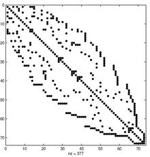
The original symmetric matrix $n\times n$ ${\ displaystyle n \ times n}$ $n\times n$ considered as a graph adjacency matrix $(V,E)$ ${\ displaystyle (V, E)}$ $(V,E)$ . The Cathill – Mackey algorithm renumbers the vertices of the graph so that, as a result of the corresponding permutation of the columns and rows of the original matrix, reduce the width of its ribbon .

The algorithm builds an ordered set of vertices $R$ ${\ displaystyle R}$ $R$ representing the new vertex numbering. For a connected graph, the algorithm is as follows:

select a peripheral vertex (or a pseudo-peripheral vertex ) $v$ ${\ displaystyle v}$ $v$ for the initial value of the tuple $R:=(v)$ ${\ displaystyle R: = (v)}$ $R:=(v)$ ;
for $i=1,2,...$ ${\ displaystyle i = 1,2, ...}$ $i=1,2,...$ while the condition is satisfied $|R|<n$ ${\ displaystyle | R | <n}$ $|R|<n$ , perform steps 3-5:
build an adjacency set $\operatorname {Adj} (R_{i})$ ${\ displaystyle \ operatorname {Adj} (R_ {i})}$ $\operatorname {Adj} (R_{i})$ for $R_{i}$ ${\ displaystyle R_ {i}}$ $R_i$ where $R_{i}$ ${\ displaystyle R_ {i}}$ $R_i$ - $i$ ${\ displaystyle i}$ $i$ component $R$ ${\ displaystyle R}$ $R$ , and exclude vertices that are already contained in $R$ ${\ displaystyle R}$ $R$ , i.e: $A_{i}:=\operatorname {Adj} (R_{i})\setminus R$ ${\ displaystyle A_ {i}: = \ operatorname {Adj} (R_ {i}) \ setminus R}$ $A_{i}:=\operatorname {Adj} (R_{i})\setminus R$ ;
sort $A_{i}$ ${\ displaystyle A_ {i}}$ $A_{i}$ ascending degrees of peaks ;
add $A_{i}$ ${\ displaystyle A_ {i}}$ $A_{i}$ in the result tuple $R$ ${\ displaystyle R}$ $R$ .

In other words, the algorithm numbers the vertices during the breadth-first search , at which adjacent vertices are dispensed in the order of increasing their degrees .

For a disconnected graph, the algorithm can be applied separately to each connected component ^[1] .

The temporal computational complexity of the RCM algorithm, provided that sorting by inserts is used for ordering, $O(m|E|)$ ${\ displaystyle O (m | E |)}$ $O(m|E|)$ where $m$ ${\ displaystyle m}$ $m$ - maximum degree of apex, $|E|$ ${\ displaystyle | E |}$ $|E|$ - the number of edges of the graph ^[2] .

Selecting the starting vertex

To get good results, you need to find the peripheral vertex of the graph. $(V,E)$ ${\ displaystyle (V, E)}$ . This task is generally quite difficult, therefore, they usually look for a pseudo-peripheral vertex using one of the modifications of the Gibbs heuristic algorithm , etc.

To describe the algorithm, the concept of a root level structure is introduced. For a given vertex $v$ ${\ displaystyle v}$ level structure with root in $v$ ${\ displaystyle v}$ will be a split ${\mathcal {L}}$ ${\ displaystyle {\ mathcal {L}}}$ many vertices $V$ ${\ displaystyle V}$ :

{\mathcal {L}}(v)=\{L_{0}(v),L_{1}(v),\dots ,L_{l(v)}(v)\},

{\ displaystyle {\ mathcal {L}} (v) = \ {L_ {0} (v), L_ {1} (v), \ dots, L_ {l (v)} (v) \},}

where are the subsets $L_{i}(v)$ ${\ displaystyle L_ {i} (v)}$ defined as follows:

L_{0}(v)=\{v\},

{\ displaystyle L_ {0} (v) = \ {v \},}

L_{1}(v)=\operatorname {Adj} (L_{0}(v))

{\ displaystyle L_ {1} (v) = \ operatorname {Adj} (L_ {0} (v))}

and

L_{i}(v)=\operatorname {Adj} (L_{i-1}(v))-L_{i-2}(v),\qquad i=2,3,\dots ,l(v).

{\ displaystyle L_ {i} (v) = \ operatorname {Adj} (L_ {i-1} (v)) - L_ {i-2} (v), \ qquad i = 2,3, \ dots, l (v).}

Algorithm for finding a pseudo-peripheral vertex ^[3] :

select arbitrary vertex $r$ ${\ displaystyle r}$ of $V$ ${\ displaystyle V}$ ;
build a level structure for the root $r$ ${\ displaystyle r}$ : ${\mathcal {L}}(r)=\{L_{0}(r),L_{1}(r),\dots ,L_{l(r)}(r)\}$ ${\ displaystyle {\ mathcal {L}} (r) = \ {L_ {0} (r), L_ {1} (r), \ dots, L_ {l (r)} (r) \}}$ ;
pick the top with the least degree $v$ ${\ displaystyle v}$ of $L_{l(r)}(r)$ ${\ displaystyle L_ {l (r)} (r)}$ ;
build a level structure for the root $v$ ${\ displaystyle v}$ : ${\mathcal {L}}(v)=\{L_{0}(v),L_{1}(v),\dots ,L_{l(v)}(v)\}$ ${\ displaystyle {\ mathcal {L}} (v) = \ {L_ {0} (v), L_ {1} (v), \ dots, L_ {l (v)} (v) \}}$ ;
if a $l(v)>l(r)$ ${\ displaystyle l (v)> l (r)}$ then assign $r:=v$ ${\ displaystyle r: = v}$ and go to step 3;
vertex $v$ ${\ displaystyle v}$ is the desired pseudo-peripheral vertex.

Notes

↑ George, Liu, 1984 , pp. 65-66.
↑ George, Liu, 1984 , p. 68.
↑ George, Liu, 1984 , pp. 70-72.

Literature

E. Cuthill and J. McKee. Reducing the bandwidth of sparse symmetric matrices In Proc. 24th Nat. Conf. ACM , pages 157-172, 1969.
George A., Liu J. Numerical solution of large sparse systems of equations = Computer Solution of Large Sparse Positive Definite Systems. - M .: Mir, 1984. - 333 p.

Links

Cuthill-Mackey documentation for Boost C ++ libraries .
Detailed explanation of the Cuthill-Mackey algorithm .
A detailed explanation of the Cathill-Mackey algorithm (Russian) (inaccessible link) .
Python Cuthill-Mackey algorithm implementation (inaccessible link) .

[_12e24bbb5ce8ef62-1] George, Liu, 1984 , pp. 65-66.

[_a57da192859561bc-2] George, Liu, 1984 , p. 68.

[_8c56bdc1ea07832f-3] George, Liu, 1984 , pp. 70-72.