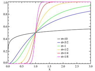
The lognormal distribution in probability theory is a two-parameter family of absolutely continuous distributions . If a random variable has a lognormal distribution, then its logarithm has a normal distribution .
| Lognormal | |
|---|---|
 μ = 0 Probability Density | |
 μ = 0 distribution function | |
| Designation | , |
| Options | |
| Carrier | |
| Probability density | |
| Distribution function | |
| Expected value | |
| Median | |
| Fashion | |
| Dispersion | |
| Asymmetry coefficient | |
| Excess ratio | |
| Differential entropy | |
| The generating function of moments | |
| Characteristic function | |
Content
Definition
Let the distribution of a random variable is given by the probability density , having the form:
Where . Then they say that has a lognormal distribution with parameters and . They write: .
Moments
Formula for of the lognormal random variable has the form:
whence in particular:
- ,
- .
Any off-center moments of the n-dimensional joint lognormal distribution can be calculated using a simple formula:
- where and - parameters of multidimensional joint distribution. Is a vector whose components determine the order of the moment. (For example, in the two-dimensional case, - the second off-center moment of the first component, - mixed second moment). Parentheses denote a scalar product.
Lognormal Distribution Properties
- If a Are independent lognormal random variables such that , then their product is also lognormal:
- .
Relationship with other distributions
- If a then .
And vice versa, if then .
Modeling Lognormal Random Variables
For modeling, a link with a normal distribution is usually used. Therefore, it is enough to generate a normally distributed random variable, for example, using the Box-Muller transform , and calculate its exponent.
Variations generalization
Lognormal distribution is a special case of the so-called Captain distribution .
Applications
The lognormal distribution satisfactorily describes the distribution of particle frequencies by their sizes during random crushing, for example hailstones in a hail , etc. However, there are exceptions, for example, the size distribution of asteroids in the solar system has a logarithmic distribution .
Literature
- Crow, Edwin L. & Shimizu, Kunio (Editors) (1988), Lognormal Distributions, Theory and Applications , vol. 88, Statistics: Textbooks and Monographs, New York: Marcel Dekker, Inc., p. xvi + 387, ISBN 0-8247-7803-0
- Aitchison, J. and Brown, JAC (1957) The Lognormal Distribution , Cambridge University Press.
- Limpert, E; Stahel, W; Abbt, M. Lognormal distributions across the sciences: keys and clues (English) // BioScience : journal. - 2001. - Vol. 51 , no. 5 . - P. 341-352 . - DOI : 10.1641 / 0006-3568 (2001) 051 [0341: LNDATS] 2.0.CO; 2 .
- Eric W. Weisstein et al. Log Normal Distribution at MathWorld . Electronic document, retrieved October 26, 2006.
- Holgate, P. The lognormal characteristic function (neopr.) // Communications in Statistics - Theory and Methods. - 1989. - T. 18 , No. 12 . - S. 4539–4548 . - DOI : 10.1080 / 03610928908830173 .
- Brooks, Robert; Corson, Jon; Donal, Wales . The Pricing of Index Options When the Underlying Assets All Follow a Lognormal Diffusion // Advances in Futures and Options Research: journal. - 1994. - Vol. 7 .


![\ exp \ left (- \ left. \ left [{\ frac {\ ln (x) - \ mu} {\ sigma}} \ right] ^ {2} \ right / 2 \ right) \ left / \ left ( x \ sigma {\ sqrt {2 \ pi}} \ right) \ right.](https://wikimedia.org/api/rest_v1/media/math/render/svg/2a9cd9248908addfd55276590f3d8102ef53ccbf)
![{\ frac {1} {2}} + {\ frac {1} {2}} {\ mathrm {Erf}} \ left [{\ frac {\ ln (x) - \ mu} {\ sigma {\ sqrt {2}}}} \ right]](https://wikimedia.org/api/rest_v1/media/math/render/svg/1a9d6e18da5576e1e9e9ebfb992655a16fd71de4)


![\ operatorname {E} [X ^ {s}] = e ^ {{s \ mu + {\ tfrac {1} {2}} s ^ {2} \ sigma ^ {2}}}.](https://wikimedia.org/api/rest_v1/media/math/render/svg/b057cd47638eaec6d974d7b4adc678cae15fa1cf)
