Euler method

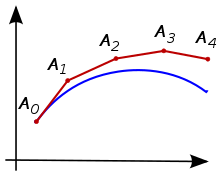
Euler's method is the simplest numerical method for solving systems of ordinary differential equations . First described by Leonard Euler in 1768 in the work “Integral Calculus” ^[1] . Euler's method is an explicit, one-step method of the first order of accuracy. It is based on approximation of the integral curve by a piecewise linear function, the so-called Euler broken line.

Euler polyline (red line) - an approximate solution in five nodes of the Cauchy problem and the exact solution to this problem (highlighted in blue)

Content

Method Description

Let the Cauchy problem for the first order equation be given:

${\frac {dy}{dx}}=f(x,y),$ ${\ displaystyle {\ frac {dy} {dx}} = f (x, y),}$

$y_{|_{x=x_{0}}}=y_{0},$ ${\ displaystyle y_ {| _ {x = x_ {0}}} = y_ {0},}$

where is the function $f$ ${\ displaystyle f}$ defined on some area $D\subset \mathbb {R} ^{2}$ {\ displaystyle D \ subset \ mathbb {R} ^ {2}} . The solution is sought on the interval $(x_{0},b]$ ${\ displaystyle (x_ {0}, b]}$ . At this interval, we introduce the nodes:

$x_{0}<x_{1}<\dots <x_{n}\leq b.$ ${\ displaystyle x_ {0} <x_ {1} <\ dots <x_ {n} \ leq b.}$

Approximate solution in nodes $x_{i}$ ${\ displaystyle x_ {i}}$ which we denote by $y_{i}$ ${\ displaystyle y_ {i}}$ is determined by the formula:

$y_{i}=y_{i-1}+(x_{i}-x_{i-1})f(x_{i-1},y_{i-1}),\quad i=1,2,3,\dots ,n.$ ${\ displaystyle y_ {i} = y_ {i-1} + (x_ {i} -x_ {i-1}) f (x_ {i-1}, y_ {i-1}), \ quad i = 1 , 2,3, \ dots, n.}$

These formulas are directly generalized to the case of systems of ordinary differential equations.

Estimation of the error of the method on the step and in the whole

The error at the step or local error is the difference between the numerical solution after one step of the calculation $y_{i}$ ${\ displaystyle y_ {i}}$ and accurate solution at the point $x_{i}=x_{i-1}+h$ ${\ displaystyle x_ {i} = x_ {i-1} + h}$ . The numerical solution is given by the formula

y_{i}=y_{i-1}+hf(x_{i-1},y_{i-1}).\quad

{\ displaystyle y_ {i} = y_ {i-1} + hf (x_ {i-1}, y_ {i-1}). \ quad}

The exact solution can be decomposed into a Taylor series :

y(x_{i-1}+h)=y(x_{i-1})+hy'(x_{i-1})+O(h^{2}).

{\ displaystyle y (x_ {i-1} + h) = y (x_ {i-1}) + hy '(x_ {i-1}) + O (h ^ {2}).}

Local error $L$ ${\ displaystyle L}$ we obtain, subtracting from the second equality the first:

L=y(x_{i-1}+h)-y_{i}=O(h^{2}).

{\ displaystyle L = y (x_ {i-1} + h) -y_ {i} = O (h ^ {2}).}

This is true if $y$ ${\ displaystyle y}$ has a continuous second derivative ^[2] . Another sufficient condition for the validity of this estimate, from which the previous one follows and which can usually be easily verified, is continuous differentiability. $f(x,y)$ ${\ displaystyle f (x, y)}$ by both arguments ^[3] .

The total error, global or cumulative error is the error at the last point of an arbitrary finite segment of integration of the equation. To calculate the solution at this point is required $S/h$ ${\ displaystyle S / h}$ steps where $S$ ${\ displaystyle S}$ length of the segment. Therefore, the global error of the method $G=O(h^{2}S/h)=O(h)$ ${\ displaystyle G = O (h ^ {2} S / h) = O (h)}$ .

Thus, the Euler method is a first order method - it has an error at the step $O(h^{2})$ ${\ displaystyle O (h ^ {2})}$ and error in general $O(h)$ ${\ displaystyle O (h)}$ ^[3] .

The value of the Euler method

The Euler method was historically the first method for the numerical solution of the Cauchy problem. O. Cauchy used this method to prove the existence of a solution to the Cauchy problem. Due to low accuracy and computational instability, the Euler method is rarely used to find solutions for the Cauchy problem in practice. However, due to its simplicity, the Euler method finds its application in theoretical studies of differential equations, variational calculus problems , and a number of other mathematical problems.

Modifications and generalizations

Modified Euler method with recalculation

To improve the accuracy and stability of the calculation of the solution, you can use the following implicit Euler method.

Forecast:

${\tilde {y}}_{i}=y_{i-1}+(x_{i}-x_{i-1})f(x_{i-1},y_{i-1})$ ${\ displaystyle {\ tilde {y}} _ {i} = y_ {i-1} + (x_ {i} -x_ {i-1}) f (x_ {i-1}, y_ {i-1} )}$ .

Correction:

$y_{i}=y_{i-1}+(x_{i}-x_{i-1}){\frac {f(x_{i-1},y_{i-1})+f(x_{i},{\tilde {y}}_{i})}{2}}$ ${\ displaystyle y_ {i} = y_ {i-1} + (x_ {i} -x_ {i-1}) {\ frac {f (x_ {i-1}, y_ {i-1}) + f (x_ {i}, {\ tilde {y}} _ {i})} {2}}}$ .

To improve accuracy, the corrective iteration can be repeated by substituting ${\tilde {y}}_{i}=y_{i}$ ${\ displaystyle {\ tilde {y}} _ {i} = y_ {i}}$ .

The modified Euler method with recalculation has a second order of accuracy, but for its implementation it is necessary to calculate at least twice $f(x,y)$ ${\ displaystyle f (x, y)}$ . The Euler method with recalculation is a type of Runge-Kutta method (predictor-corrector).

Adams – Bashfort Two-Step Method

Another way to improve the accuracy of the method is to use not one, but several previously calculated function values:

y_{i+1}=y_{i}+{\tfrac {3}{2}}hf(x_{i},y_{i})-{\tfrac {1}{2}}hf(x_{i-1},y_{i-1}).

{\ displaystyle y_ {i + 1} = y_ {i} + {\ tfrac {3} {2}} hf (x_ {i}, y_ {i}) - {\ tfrac {1} {2}} hf ( x_ {i-1}, y_ {i-1}).}

This is a linear multi-step method .

Implementations in programming languages

C implementation for function $f(x,y)=6x^{2}+5xy$ {\ displaystyle f (x, y) = 6x ^ {2} + 5xy} .

  #include <stdio.h> 

 double func ( double x , double y )
 {
	 return 6 * x * x + 5 * x * y ;  // function of the first derivative
 }

 int main ( int argc , char ** argv )
 {
     int i , n ; 
     double x , y , h ;

     h = 0.01 ;  // step
     n = 10 ;  // number of iterations
     x = 1 ;  // x0
     y = 1 ;  // y0

     for ( i = 0 ; i < n ; i ++ )
     {
         y + = h * func ( x , y );  // calculate yi
         x + = h ;
     }

     return EXIT_SUCCESS ;
 }

Implementation in Python 3.7 :

  # n is the number of iterations, h is the step, (x, y) is the starting point
 def Euler ( n = 10 , h = 0.01 , x = 1 , y = 1 ):
     for i in range ( n ):
         y + = h * function ( x , y )
         x + = h
     return x , y # solution

 def function ( x , y ):
     return 6 * x ** 2 + 5 * x * y # function of the first derivative

 print ( Euler ())

Literature

Euler L. Integral calculus. Volume 1. - M .: Hittl. 1956. [1]
Babenko K.I. Fundamentals of numerical analysis. - M .: Science. 1986

Notes

↑ Euler L. Integral Calculus, Volume 1, Section 2, Ch. 7
↑ Atkinson, Kendall A. (1989), An Introduction to Numerical Analysis (2nd ed.), New York: John Wiley & Sons , p. 342, ISBN 978-0-471-50023-0
↑ ¹ ² Mathematical Encyclopedic Dictionary. - M .: “Owls. Encyclopedia " , 1988. - p. 641.

[1] Euler L. Integral Calculus, Volume 1, Section 2, Ch. 7

[2] Atkinson, Kendall A. (1989), An Introduction to Numerical Analysis (2nd ed.), New York: John Wiley & Sons , p. 342, ISBN 978-0-471-50023-0

[МЭС-3] ¹ ² Mathematical Encyclopedic Dictionary. - M .: “Owls. Encyclopedia " , 1988. - p. 641.